0. Why R?

It's free, and SAS/STATA/SPSS ain't
When in rome. It's the language that 'real' statisticians use.
Community. Great support for many arcane things.
Graphics. Lots of options. Start with GGPlot2 ?

1. Why not R?

It can be a pain. You can do a lot of stats with Excel. Postgres ships with standard deviation for goodness sakes.
If all you have is a hammer... Many of R's simpler functions can be achieved with a programming language. With python, try numpy/scipy ; or an explicit python based R alternative called PANDAS (not to be confused with the knight challenge winner, which is singular).
Really big data. R likes to read everything into memory, so if you've got gigabyte data-sets it might not be ideal.

2. OK, it sounds good, but I hate the command line

I'm not gonna talk about it, but check out R commander which attempts to make R work with a GUI. It might suck, I don't know
Also see R Excel, which allows you to do stuff from Excel. Also, don't know if it works.

3. I'm a bad-ass programmer running a monstrous horde of news apps. I don't wanna do anything outside ruby.

No worries, R has libraries that allow you to execute stuff from python with RPy2 and in Ruby. Not sure what's best in Ruby--maybe try RSruby. Lemme know if it works...
R is itself a programming language, of course. So maybe you should do your coding in there.
Fun fact: entering a function without the parenthesis will show the source code. Entering "cor(somedata)" will run a correlation -- but entering just "cor" will show you the source code. Super handy to figure out how stuff works.

4. Disclaimer - Running with scissors

There's no alternative to actually knowing stats. Learn 'em. The more equations the better. Knowing stats without reading the equations is like learning to drive without ever getting into a car.
If you're not sure, get professional help. Junior faculty members can be a good place to start.

5. Fire up R

If you're following along at home jump to installation.

It's in the applications thingy on windows in the lab machines. I couldn't find it either. $@#$ Windows.
Just in case you're wondering, it does look like crap on windows. There also appear to be some odd permissions.
Where are we in the filesystem? We're doing this to figure out how to deal with filepaths on windows machines, so it'll look a bit different. The '>' lines are the input lines.
¡ ¡ The file paths in the labs will be different--I'm just doing this as an example
```
    > getwd()
    [1] "/Users/ruser"
    > setwd('/Users/ruser/nicar-stlouis/r-presentation')
    >	    
            
    	
```
Get a sample file of selected census summary-level 140 demographics. From the 05-09 ACS y'all: http://jacobfenton.s3.amazonaws.com/county_demographics.txt
It's a good idea to eyeball the file and see what's going on. This file is pretty clean--consistent quotes, tab delimited, and missing values are just missing. The tabs might not be apparent, but they're in there. Look for "Prince of Wales-Outer Ketchikan". (Can anyone tell me why the file is misleadingly named? It's really 140... )
Save the file somewhere in the filesystem, if you haven't already, so you can load it up.

    > # check it out we can write comment characters in R too
    > # I'm loading the file with a header row, with the column 
    > # separator set to be a tab, and with quotes as quotes. 
    > counties <- read.delim("/path/to/your/file/county_demographics.txt",header=TRUE, sep="\t", quote='"')
    > # What are the column names? 
    > colnames(counties)
    [1] "state"            "co"               "pop"              "median_hh_income" "ba_plus"          "white_pcnt"       "black_pcnt"      
    [8] "hispanic_pcnt"    "pov_pcnt"
    > # This is a bit odd, but this data is now stored in R as a 'data frame'. Don't worry about this for the moment. 
    > # Here's how we access data in a data frame: 
    > counties$state

    > summary(counties$state)
       Ala.  Alaska   Ariz.    Ark.  Calif.   Colo.   Conn.    D.C.    Del.     Fla     Ga.  Hawaii   Idaho    Ill.    Ind.    Iowa  Kansas     Ky. 
         67      27      15      75      58      63       8       1       3      67     159       5      44     102      92      99     105     120 
        La.   Maine   Mass.     Md.   Mich.   Minn.   Miss.     Mo.   Mont. N. Dak. N. Mex.    N.C.    N.H.    N.J.    N.Y.    Neb.    Nev.    Ohio 
         64      16      14      24      83      87      82     115      56      53      33     100      10      21      62      93      17      88 
      Okla.    Ore.     Pa.    R.I.    S.C.    S.D.   Tenn.   Texas    Utah     Va.     Vt.  W. Va.   Wash.    Wis.    Wyo. 
         77      36      67       5      46      66      95     254      29     134      14      55      39      72      23

    > summary(counties)
         state                   co            pop          median_hh_income    ba_plus        white_pcnt    
     Texas  : 254   Washington Co.:  30   Min.   :     78   Min.   : 18869   Min.   : 5.00   Min.   :  6.00  
     Ga.    : 159   Jefferson Co. :  25   1st Qu.:  11011   1st Qu.: 35979   1st Qu.:13.00   1st Qu.: 77.00  
     Va.    : 134   Franklin Co.  :  24   Median :  25436   Median : 41652   Median :17.00   Median : 90.00  
     Ky.    : 120   Jackson Co.   :  23   Mean   :  96077   Mean   : 43435   Mean   :18.68   Mean   : 83.92  
     Mo.    : 115   Lincoln Co.   :  23   3rd Qu.:  65524   3rd Qu.: 48285   3rd Qu.:22.00   3rd Qu.: 96.00  
     Kansas : 105   Madison Co.   :  19   Max.   :9785295   Max.   :113313   Max.   :69.00   Max.   :100.00  
     (Other):2253   (Other)       :2996   NA's   :      3   NA's   :     3   NA's   : 3.00   NA's   :  3.00  
       black_pcnt      hispanic_pcnt       pov_pcnt    
     Min.   :  0.000   Min.   : 0.000   Min.   : 1.00  
     1st Qu.:  1.000   1st Qu.: 1.000   1st Qu.:11.00  
     Median :  3.000   Median : 3.000   Median :14.00  
     Mean   :  9.618   Mean   : 7.623   Mean   :15.27  
     3rd Qu.: 12.000   3rd Qu.: 7.000   3rd Qu.:19.00  
     Max.   : 87.000   Max.   :99.000   Max.   :47.00  
     NA's   :252.000   NA's   :46.000   NA's   : 5.00

¡ ¡ Malformed data files with unclosed quotes will confuse R--typically resulting in fewer lines than expected. So it's a good idea to check that all your rows got there.

    > # how many rows are in the data altogether? 
    > nrow(counties)
    [1] 3140

    > # lets copy the counties
    > counties2 <- counties

    > # lets change units in income. What did I say income was again?
    > colnames(counties2)
    [1] "state"            "co"               "pop"              "median_hh_income" "ba_plus"          "white_pcnt"      
    [7] "black_pcnt"       "hispanic_pcnt"    "pov_pcnt"        
    > # right, it's median_hh_income, (Good ole B19013 for census peeps)
    > counties2$income = counties2$median_hh_income/1000
    > # did it work? 
    > counties2$income[0]
    numeric(0)
    # Whoa--that's not what you might have been expecting
    # The zeroeth entry tells us the data type. 
    # In other words, the columns that are the data are 1-indexed
    # Let's see the first row:
    > counties2$income[1]
    [1] 51.463
    > counties$median_hh_income[1]
    [1] 51463

6. Do some basic viz

I sure hope this works out in the labs.

Run a histogram of the median income.

    > hist(counties$median_hh_income)

You should see something like this:

Here's how to print out the graphic to a file:

    > png("median_income.png", width=500, height=300, units="px")
    > hist(counties$median_hh_income)
    > # Now turn the graphic output off
    > dev.off()
    quartz 
         2 
    > # wait, where did it go? 
    > getwd()
    [1] "/path/to/where/the/png/is/now"
    >

7. Side track: what the heck is c

Data comes in columns. So it shouldn't be a surprise that we use columns to tell R how to do stuff to.

    > # lets count up to 10
    > c(1:10)
     [1]  1  2  3  4  5  6  7  8  9 10
    > # we can do math too:
    > c(10*1:10+1)
     [1]  11  21  31  41  51  61  71  81  91 101
    > # or even use text
    > c("poisson", "binomial")
    [1] "poisson"  "binomial"

8. Style the chart a bit more

This stuff can be a bit cryptic--see the docs

    > hist(counties$median_hh_income/1000,breaks=c (0:100,1000), xlim=c(0,90), 
freq=TRUE, xlab="Income, $000", main="Median income by county equivalent")
    Warning message:
    In plot.histogram(r, freq = freq1, col = col, border = border, angle = angle,  :
      the AREAS in the plot are wrong -- rather use freq=FALSE
    >

Ignore the warning message--it's referring to a part of the chart that we can't see.

I'm not gonna explain this too much. But basically we're creating a column that tells it where the breaks--the borders between histogram bins should be are, then telling it a column of the x-minimum and maximum views are, giving the x-axis a label (xlab) and the chart a title. Why is the title the "main" variable. I have no idea!

Relationships between the data

9. Look at the data more

R's plot command is pretty robust. Lets get to it.

   > plot(counties$median_hh_income, counties$ba_plus)

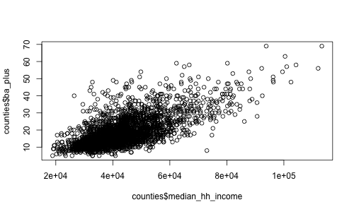
So there's obviously a relationship there. How much?

    > cor(counties$median_hh_income, counties$ba_plus)
    [1] NA
    > # We can't correlate because there are null values.
    > cor(counties$median_hh_income, counties$ba_plus, use="complete.obs")
    [1] 0.6763103

In the above, we're just saying use only the complete observations. That could be dangerous.
Also note--the default is pearson correlation. But sometimes it's useful to use spearman (rank)

    > cor(counties$median_hh_income, counties$ba_plus, use="complete.obs", method='pearson')
    [1] 0.6763103
    > cor(counties$median_hh_income, counties$ba_plus, use="complete.obs", method='spearman')
    [1] 0.6236564

What about the uncertainty of the correlation?

     > cor.test(counties$median_hh_income, counties$ba_plus, use="complete.obs")

     	Pearson's product-moment correlation

     data:  counties$median_hh_income and counties$ba_plus 
     t = 51.4071, df = 3135, p-value < 2.2e-16
     alternative hypothesis: true correlation is not equal to 0 
     95 percent confidence interval:
      0.6568609 0.6948604 
     sample estimates:
           cor 
     0.6763103 

     >

But we're only examining one relationship this way. Lets do all of them. I'm gonna transform it into a matrix. Don't ask why, I'm not really sure.

    > county_matrix <- data.matrix(counties)
    > cor(county_matrix, use="complete.obs")
                           state           co         pop median_hh_income      ba_plus
    state             1.00000000  0.013705958 -0.05401844       0.03493939  0.035086788
    co                0.01370596  1.000000000  0.01460693       0.02956972  0.004772263
    pop              -0.05401844  0.014606927  1.00000000       0.26945683  0.325710503
    median_hh_income  0.03493939  0.029569722  0.26945683       1.00000000  0.685827752
    ba_plus           0.03508679  0.004772263  0.32571050       0.68582775  1.000000000
    white_pcnt        0.12284483  0.002043147 -0.17966726       0.13377545  0.013097471
    black_pcnt       -0.12748272 -0.008496116  0.06352790      -0.23045513 -0.097418256
    hispanic_pcnt     0.08728682  0.028717294  0.18910339       0.01684250  0.020222111
    pov_pcnt         -0.06326769 -0.014163910 -0.13208919      -0.79398962 -0.432999042
                       white_pcnt   black_pcnt hispanic_pcnt    pov_pcnt
    state             0.122844834 -0.127482722    0.08728682 -0.06326769
    co                0.002043147 -0.008496116    0.02871729 -0.01416391
    pop              -0.179667258  0.063527896    0.18910339 -0.13208919
    median_hh_income  0.133775455 -0.230455130    0.01684250 -0.79398962
    ba_plus           0.013097471 -0.097418256    0.02022211 -0.43299904
    white_pcnt        1.000000000 -0.832365355   -0.15548590 -0.41024198
    black_pcnt       -0.832365355  1.000000000   -0.11994898  0.42466780
    hispanic_pcnt    -0.155485898 -0.119948976    1.00000000  0.09953580
    pov_pcnt         -0.410241980  0.424667802    0.09953580  1.00000000

That's hard to read, lets write it out to a table in the filesystem:

    > cor_found <- cor(county_matrix, use="complete.obs")
    > write.table( cor_found, file="correlations.txt", sep="|", eol="\n", row.names=TRUE)

state co pop income ba_plus white_pcnt black_pcnt hispanic_pcnt pov_pcnt

state 1.00 0.01 -0.05 0.03 0.04 0.12 -0.13 0.09 -0.06

co 0.01 1.00 0.01 0.03 0.00 0.00 -0.01 0.03 -0.01

pop -0.05 0.01 1.00 0.27 0.33 -0.18 0.06 0.19 -0.13

income 0.03 0.03 0.27 1.00 0.69 0.13 -0.23 0.02 -0.79

ba_plus 0.04 0.00 0.33 0.69 1.00 0.01 -0.10 0.02 -0.43

white_pcnt 0.12 0.00 -0.18 0.13 0.01 1.00 -0.83 -0.16 -0.41

black_pcnt -0.13 -0.01 0.06 -0.23 -0.10 -0.83 1.00 -0.12 0.42

hispanic_pcnt 0.09 0.03 0.19 0.02 0.02 -0.16 -0.12 1.00 0.10

pov_pcnt -0.06 -0.01 -0.13 -0.79 -0.43 -0.41 0.42 0.10 1.00

	state	co	pop	income	ba_plus	white_pcnt	black_pcnt	hispanic_pcnt	pov_pcnt
state	1.00	0.01	-0.05	0.03	0.04	0.12	-0.13	0.09	-0.06
co	0.01	1.00	0.01	0.03	0.00	0.00	-0.01	0.03	-0.01
pop	-0.05	0.01	1.00	0.27	0.33	-0.18	0.06	0.19	-0.13
income	0.03	0.03	0.27	1.00	0.69	0.13	-0.23	0.02	-0.79
ba_plus	0.04	0.00	0.33	0.69	1.00	0.01	-0.10	0.02	-0.43
white_pcnt	0.12	0.00	-0.18	0.13	0.01	1.00	-0.83	-0.16	-0.41
black_pcnt	-0.13	-0.01	0.06	-0.23	-0.10	-0.83	1.00	-0.12	0.42
hispanic_pcnt	0.09	0.03	0.19	0.02	0.02	-0.16	-0.12	1.00	0.10
pov_pcnt	-0.06	-0.01	-0.13	-0.79	-0.43	-0.41	0.42	0.10	1.00

10. Pearson correlation is for linear correlation

Shamelessly ripped off from wikipedia

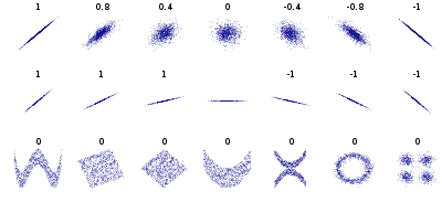
If you're looking for *non-linear* relationships use spearman correlation...

Done!

But if we're not out of time yet, here's more

11. Adding libraries

All kinds of good stuff is put out by random people (typically people who know way more about it than I). Stuff is different on windows. Here's how it works on Mac, roughly:

"Packages & Data" > "R Package Manager" lots of stuff ships with R, you might just have to load it.
on macs, click load, then, to load it at the console
```
> library(ggplot2)
```
Can load the data via repository; in macs: "Packages & Data" > "R Package Installer"

I skipped this because it varies with platform. It's pretty painless on my rig, just remember to click the 'add dependencies' button, which oddly isn't checked by default.

12. Getting help

There's a system help. It's not incredibly helpful for beginners (though it's invaluable if you really want to know how something works). You can get to it with windows. In general, typing '?command' at the console *should* launch it, but in the labs it doesn't. I could make it work by cutting a pasting the local help url--once it's started in the labs--into a browser bar.
http://127.0.0.1:10788/doc/html/index.html This might work in the labs (?)
http://127.0.0.1:10788/library/base/html/getwd.html

"Packages & Data" > "R Package Manager" lots of stuff ships with R, you might just have to load it.
on macs, click load, then, to load it at the console
```
> library(ggplot2)
```
Can load the data via repository; in macs: "Packages & Data" > "R Package Installer"
The reality is--it's usually more helpful to google for examples; try stackoverflow etc. Also, the name 'R' is totally unhelpful for googling purposes. Which is a funny problem. Try 'r statistics' + your help term.
I mentioned this before, but you can see the source code of a function by just typing it at the console window without parentheses. Not sure that's actually helpful, but...

13. Working example: dates, ggplot2, etc.

Here's a data file, call it faceted.txt

    a <- read.delim("/Users/jacobfenton/IRW/banks_small_biz/parse_custom/custom_read.csv",header=TRUE, sep=",", quote='"')

14. Installation

There are installers for Mac and for windows. Installing with homebrew to use at the command line, for example, seems to make it harder to do thing like load and install packages from remote libraries.

Intro to R

Jacob Fenton
Sunlight Foundation
jfenton@sunlightfoundation.com

This presentation is available at:
http://bit.ly/correlation-does-not-imply-causation

0. Why R?

1. Why not R?

2. OK, it sounds good, but I hate the command line

3. I'm a bad-ass programmer running a monstrous horde of news apps. I don't wanna do anything outside ruby.

4. Disclaimer - Running with scissors

5. Fire up R

6. Do some basic viz

7. Side track: what the heck is c

8. Style the chart a bit more

9. Look at the data more

10. Pearson correlation is for linear correlation

Done!

11. Adding libraries

12. Getting help

13. Working example: dates, ggplot2, etc.

14. Installation

Intro to R

Jacob Fenton Sunlight Foundation jfenton@sunlightfoundation.com

This presentation is available at: http://bit.ly/correlation-does-not-imply-causation

0. Why R?

1. Why not R?

2. OK, it sounds good, but I hate the command line

3. I'm a bad-ass programmer running a monstrous horde of news apps. I don't wanna do anything outside ruby.

4. *Disclaimer* - Running with scissors

5. Fire up R

6. Do some basic viz

7. Side track: what the heck is c

8. Style the chart a bit more

9. Look at the data more

10. Pearson correlation is for *linear* correlation

Done!

11. Adding libraries

12. Getting help

13. Working example: dates, ggplot2, etc.

14. Installation

Jacob Fenton
Sunlight Foundation
jfenton@sunlightfoundation.com

This presentation is available at:
http://bit.ly/correlation-does-not-imply-causation

4. Disclaimer - Running with scissors

10. Pearson correlation is for linear correlation